Bode plots, named after the mathematician Hendrik W. Bode, are commonly used to display frequency response plots of linear systems; in these plots, the horizontal axis represents frequency on a logarithmic scale (base 10) and the vertical axis represents the amplitude or phase of the frequency response function.
The amplitude in Bode plots is shown in dB, where

At first glance, logarithmic plots may seem overly complicated; however, they offer two major benefits.
1. Since log(ab/c) = log(a) + log(b) log(c), the product of terms in a frequency response function is a sum of terms (c). Bode (logarithmic) plots can be built from the sum of plots of individual terms, which is an advantage. Furthermore, any frequency response function will only ever have four types of terms:
- A constant K.
- Poles or zeros “at the origin”(jω).
- Simple poles or zeros (1 + jωτ) or (1 + jω/ωo).
- Quadratic poles or zeros [1+ jωτ +(jω/ωn)2].
2. The Bode plots of these four separate terms can be approximatively represented by linear segments, and these segments can be easily added together to produce the Bode plot of more complex frequency response functions.
RC Low-Pass Filter Bode Plots
Think of a low-pass filter with a resistor and capacitor. What follows is a frequency response function:

where 0 is the filter’s cutoff (or half-power) frequency and = RC = 1/0 is the circuit time constant. This FREQ function has a cutoff frequency of 0 = 1/ = 1/RC and a simple pole with a constant of value K = 1.
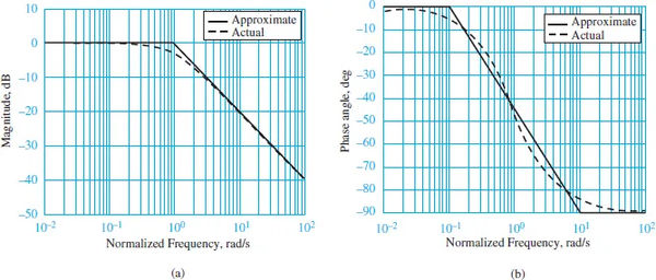
Bode magnitude and phase plots for the filter are shown in Figure 1 below.

For the horizontal axis, we have standardized frequency to. When the absolute value of the frequency response function is transformed into logarithm form, the magnitude plot is the result.

When ω ≪ ω0, the imaginary part of the simple pole is much smaller than its real part, such that |1 + jω/ω0| ≈ 1. Then:

As a result, the low-frequency asymptote of the Bode magnitude plot, which is a straight line with zero slope, can accurately approximate equation 3 at very low frequencies ( 0).
When ω ≫ ω0, the simple pole’s imaginary portion is significantly larger than its real portion, causing |1 + j/0| | j/0| = (/0). Then:

At very high frequencies (ω ≫ ω0), a straight line with a slope of 20 dB per decade that intersects the log axis at log 0 is a good approximation of equation 3. Here we see the high-frequency asymptote of the Bode magnitude plot. In terms of frequency, a decade is equivalent to a 10-fold change. As a result, a change of one in log is equivalent to a change of a decade in.
Finally, when ω = ω0, the real and imaginary parts of the simple pole are equal, such that |1 + jω/ω0| = |1 + j| =√2. Then equation 3 becomes:

For this reason, a first-order low-pass filter’s Bode magnitude plot is represented by two parallel lines that meet at zero. The approximation is illustrated in Figure 1(a). At the cutoff frequency, where = o occurs, the true Bode magnitude plot is 3 dB weaker than the approximate plot.
The phase angle of the frequency response function  has the following properties:
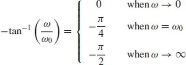
Initially, the phase angle can be represented by three parallel lines:

Figure 1 depicts these approximations using straight lines (b).
Comparison of the precise and approximate Bode magnitude and phase plots are shown in Table 1. The cutoff frequency is also referred to as the 3-dB frequency or the half-power frequency because that is where the maximum magnitude difference occurs.
Asymptotic approximation of a first-order filter: table 1 of correction factors
| ω/ω0 | Magnitude response error, (dB) | Phase response error (deg) |
| 0.1 | 0 | −5.7 |
| 0.5 | -1 | 4.9 |
| 1 | -3 | 0 |
| 2 | -1 | -4.9 |
| 10 | 0 | +5.7 |
RC High-Pass Filter Bode Plots
As with the RC low-pass filter, an RC high-pass filter is analyzed in detail. What follows is a frequency response function:
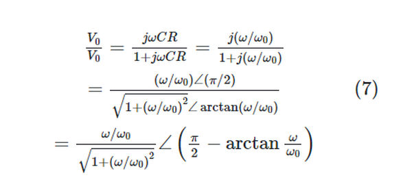
Bode plots are shown in Figure 2 for equation 7, with the normalized frequency ω/ω0 on the horizontal axis. Once again, at low and high frequencies, straight-line asymptotic approximations can be easily determined. The outcomes are comparable to those of a first-order low-pass filter.
The Bode magnitude approximation has a slope of +20 dB/decade for ω < ω0, which means that it crosses the origin ( = 1). The Bode magnitude approximation for > 0 is flat at 0 dB.
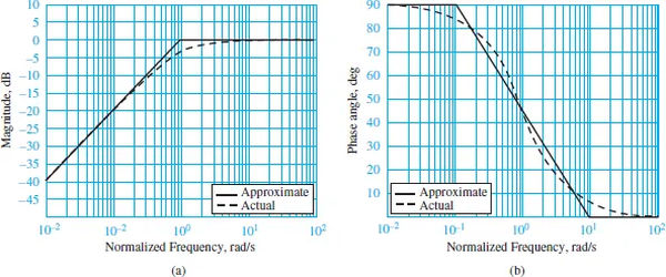
The straight- line approximations of the Bode phase plot are:

These straight-line approximations are illustrated in Figure 2(b).
Bode Plots of Higher-Order Filters
High-order system Bode plots can be constructed by summing the Bode plots of the factors that make up the system’s frequency response. For instance,

for which the logarithm is

and

To illustrate, think about the frequency response function.

Each term in the expression must be factored into the form ai (j/i +1), where I is the appropriate 3-dB frequency (1, 2, or 3), before the asymptotic approximation can be calculated. If we rewrite the function in Eq. 11 as:

Equation 12 can now be expressed in logarithmic form:

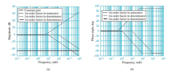
The logarithmic magnitude expression can be plotted with each term displayed separately.
In Figure 3(a), the constant is depicted as a horizontal line with a slope of 46 dB.
Figure 1(a) is a first-order Bode plot, with the numerator term expressed as a line with a slope of +20 dB/decade that leaves the zero axis at a frequency of 1 = 5; the two denominator factors are similarly expressed as lines with slopes of 20 dB/decade that leave the zero axis at a frequency of 2 = 10 and 3 = 100, respectively.
After the frequency response function has been normalized in the form of equation 9, you can easily plot the individual factors by eye.
Now that we’ve looked at the phase response part of equation 13, we know that the first term, the phase angle of the constant, is always zero.
Conversely, a straight line with a slope of +/4rad/decade (positive because this is a numerator factor) from 0.11 = 0.5 to 101 = 50 (where the asymptote is +/2) can be used to approximate the numerator first-order term.
Similar behavior is observed for both denominator terms except that the slope of the straight line between the frequencies of 0.12 and 102 and 0.13 and 103 is /4 rad/decade.
Magnitude factors are shown in Figure 3(a), and phase factors are shown in Figure 3(b), both of which depict the asymptotic approximations of the individual factors in equation 13. (b). The overall frequency response approximation can be obtained by summing all the asymptotic approximations.
Asymptotic Bode approximation results compared to measured frequency response functions are shown in Figure 4.
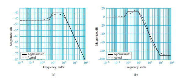
You can see that, even for higher-order frequency response functions, sketching a good approximation of the Bode plot is straightforward once the function is factored into the proper form.
Bode Plot Step by Step Guide
Here we show you how to construct an asymptotic approximation of a Bode plot. Both the numerator and denominator must be factorable into first-order terms with real roots for this method to work.
- To factorize the frequency response function yields an expression like the one below:

- To determine the range of frequencies for the semi-logarithmic plot, making sure it includes at least ten years below the lowest 3-dB frequency and at least ten years above the highest 3-dB frequency.
- Using the methods depicted in Figures 1–4, sketch the asymptotic approximations of the magnitude and phase response for each of the first-order factors.
- Add the individual terms graphically to get the total answer.
- It’s optional at this point to use Table 1’s correction factors.
